VLOOKUP in R with Schwartau Beehive Data
I started learning R back in 2016 in college thanks to a couple of my professors who used it to teach statistics: Dr. Grimshaw and Dr. Lawson. Thanks to the R community I’ve learned a lot more since then, but recently I did an embarrassing Google search for “how to do VLOOKUP in r.”
For those of you who don’t know, VLOOKUP is a function in Excel that takes two ranges, matches two of the columns, and gives you a result from a third column based on the match. There are some nuances, like that the matching column in the “from” range has to be the first one, and the difference between approximate and exact matches, but we’ll stay out of the Excel weeds on this post. Suffice it to say that dplyr merges are the ticket for 90% of what VLOOKUP gets used for and it’s way faster.
This post is largely insurance to make sure that I never do that Google search again. First, I’ll load the tidyverse (which includes dplyr) and grab some sample data. I’ll also load tibbletime to prepare the data more easily.
library(tidyverse)
library(tibbletime)
For some example data I hopped on to kaggle and grabbed a recent dataset about some behives that looked interesting. For the purpose of this exercise I’m going to calculate the average daily temperature and bee departures so that we can easily merge the two together.
temp <- read_csv("data/temperature_schwartau.csv")## Parsed with column specification:
## cols(
## timestamp = col_datetime(format = ""),
## temperature = col_double()
## )temp## # A tibble: 253,430 x 2
## timestamp temperature
## <dttm> <dbl>
## 1 2017-01-01 14:10:00 NA
## 2 2017-01-01 14:15:00 12.3
## 3 2017-01-01 14:20:00 12.3
## 4 2017-01-01 14:25:00 12.3
## 5 2017-01-01 14:30:00 12.4
## 6 2017-01-01 14:35:00 12.4
## 7 2017-01-01 14:40:00 12.5
## 8 2017-01-01 14:45:00 12.5
## 9 2017-01-01 14:50:00 12.5
## 10 2017-01-01 14:55:00 12.5
## # ... with 253,420 more rowsflow <- read_csv("data/flow_schwartau.csv")## Parsed with column specification:
## cols(
## timestamp = col_datetime(format = ""),
## flow = col_double()
## )flow## # A tibble: 2,513,836 x 2
## timestamp flow
## <dttm> <dbl>
## 1 2017-01-01 14:15:00 0
## 2 2017-01-01 14:16:00 0
## 3 2017-01-01 14:17:00 0
## 4 2017-01-01 14:18:00 0
## 5 2017-01-01 14:19:00 0
## 6 2017-01-01 14:20:00 0
## 7 2017-01-01 14:21:00 0
## 8 2017-01-01 14:22:00 0
## 9 2017-01-01 14:23:00 0
## 10 2017-01-01 14:24:00 0
## # ... with 2,513,826 more rowsTo get the data ready for this demo I’m going to take the hourly average flow out of the hive (positive values) and the hourly average temperature.
flow <- flow %>%
  drop_na() %>%
  mutate(exit_flow = case_when( # get only departures
    flow >= 0 ~ flow
  )) %>%
  drop_na() %>% # drop all arriving rows
  arrange(timestamp) %>% # tble_time needs the timestamp to be ordered
  tbl_time(index = timestamp) %>% # convert to tble_time for ease of grouping by hour
  collapse_by(period = "hourly", clean = TRUE) %>% # "collapse" by hour
  group_by(timestamp) %>% # group by collapsed hourly column
  summarise(mean_exit_flow = mean(exit_flow)) # get the hourly average
flow
## # A time tibble: 20,953 x 2
## # Index: timestamp
## timestamp mean_exit_flow
## <dttm> <dbl>
## 1 2017-01-01 15:00:00 0
## 2 2017-01-01 16:00:00 0
## 3 2017-01-01 17:00:00 0
## 4 2017-01-01 18:00:00 0
## 5 2017-01-01 19:00:00 0.00847
## 6 2017-01-01 20:00:00 0
## 7 2017-01-01 21:00:00 0
## 8 2017-01-01 22:00:00 0
## 9 2017-01-01 23:00:00 0
## 10 2017-01-02 00:00:00 0
## # ... with 20,943 more rowstemp <- temp %>%
drop_na() %>%
arrange(timestamp) %>%
tbl_time(index = timestamp) %>%
collapse_by(period = "hourly", clean = TRUE) %>%
group_by(timestamp) %>%
summarise(mean_temp = mean(temperature))
temp## # A time tibble: 20,953 x 2
## # Index: timestamp
## timestamp mean_temp
## <dttm> <dbl>
## 1 2017-01-01 15:00:00 12.4
## 2 2017-01-01 16:00:00 13.4
## 3 2017-01-01 17:00:00 16.7
## 4 2017-01-01 18:00:00 16.4
## 5 2017-01-01 19:00:00 13.7
## 6 2017-01-01 20:00:00 14.0
## 7 2017-01-01 21:00:00 12.4
## 8 2017-01-01 22:00:00 17.3
## 9 2017-01-01 23:00:00 17.8
## 10 2017-01-02 00:00:00 20.0
## # ... with 20,943 more rowsYou can see that the first column of both tables match exactly, with one row for each hour and the right column of each table do not match. This is one scenario that I might use VLOOKUP for in Excel, especially if the data isn’t ordered, or if I don’t know if both datasets are complete.
As a side note, the flow dataset has 2.5 million rows and the temperature dataset has 250 thousand rows. Summarizing these by hour into tables of about 21 thousand rows and then combining them would be a trying task for Excel, but for R it’s a breeze.
To combine these two in R, I will use a join function from dplyr. VLOOKUP works like left_join() or right_join() because it looks for matches from one table in another table. If there aren’t any matches, it returns with an error. We also have the option to do a full_join() which returns all rows from both tables and with NA wherever there isn’t a match or inner_join() which only returns rows where there are matches from both tables.
Since I have created a nice clean dataset with matching timestamp columns, I will get the same result no matter which join function I use. dplyr will try to guess which column I want to join by and return its guess as a message unless I specify which column I want it to use with by =.
joined_table <- flow %>%
  left_join(temp, by = "timestamp")
joined_table
## # A time tibble: 20,953 x 3
## # Index: timestamp
## timestamp mean_exit_flow mean_temp
## <dttm> <dbl> <dbl>
## 1 2017-01-01 15:00:00 0 12.4
## 2 2017-01-01 16:00:00 0 13.4
## 3 2017-01-01 17:00:00 0 16.7
## 4 2017-01-01 18:00:00 0 16.4
## 5 2017-01-01 19:00:00 0.00847 13.7
## 6 2017-01-01 20:00:00 0 14.0
## 7 2017-01-01 21:00:00 0 12.4
## 8 2017-01-01 22:00:00 0 17.3
## 9 2017-01-01 23:00:00 0 17.8
## 10 2017-01-02 00:00:00 0 20.0
## # ... with 20,943 more rowsPretty easy! Preparing this dataset took more work than joining it, but there are a lot of cases where the data will lend itself to a join right out of the box.
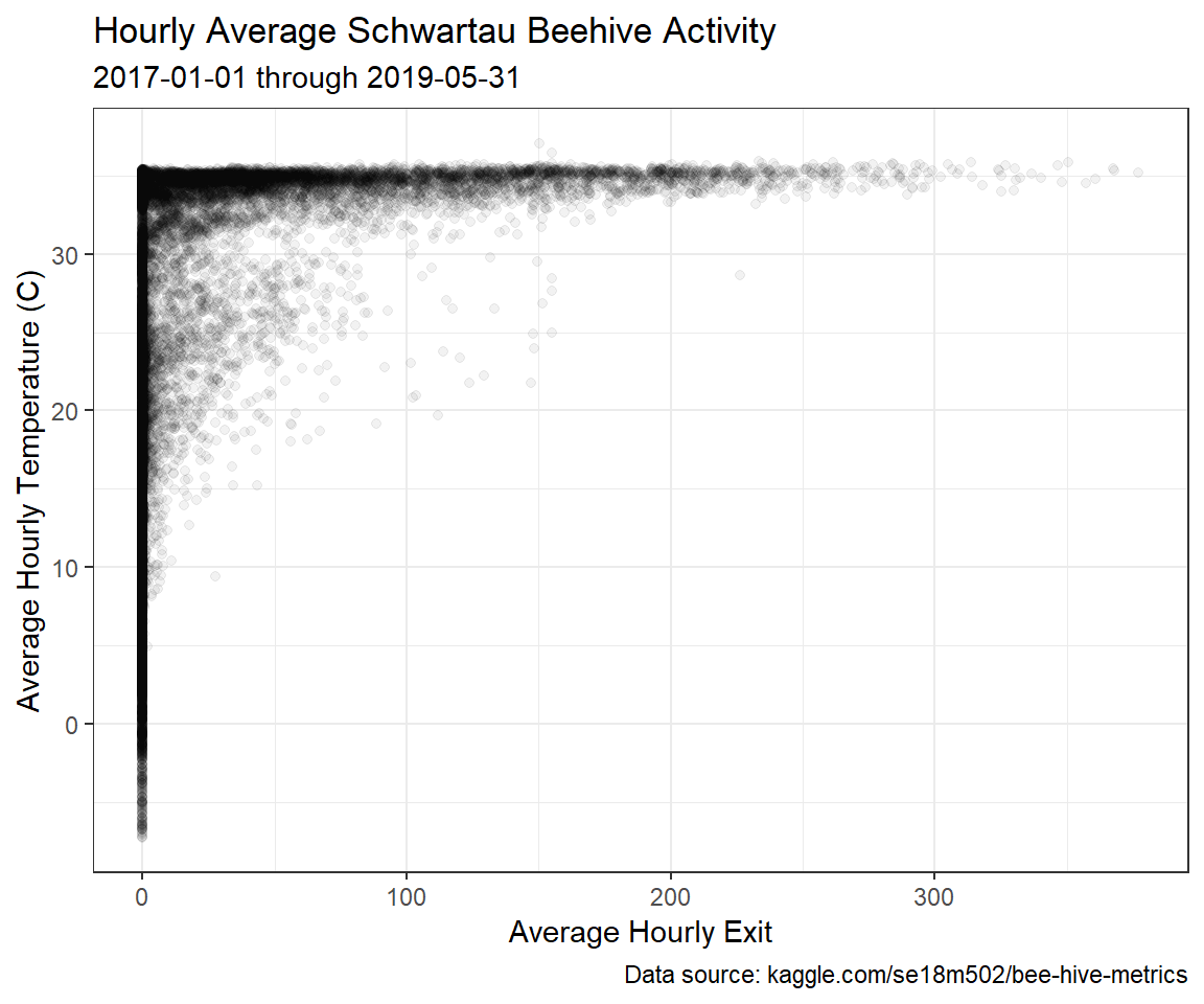
Since we’ve made it this far, let’s take a look at the relationship between the hourly average number of bees exiting the hive and the hourly average temperature.
joined_table %>%
  ggplot(aes(x = mean_exit_flow, y = mean_temp)) +
  geom_point(alpha = .05) +
  labs(title = "Hourly Average Schwartau Beehive Activity", subtitle = "2017-01-01 through 2019-05-31", caption = "Data source: kaggle.com/se18m502/bee-hive-metrics") +
  xlab("Average Hourly Exit") +
  ylab("Average Hourly Temperature (C)") +
  theme_bw()
It looks like it needs to be about 10 C (50 F) before these bees want to head outdoors, and above 30 C (86 F) there is a huge spike in activity.
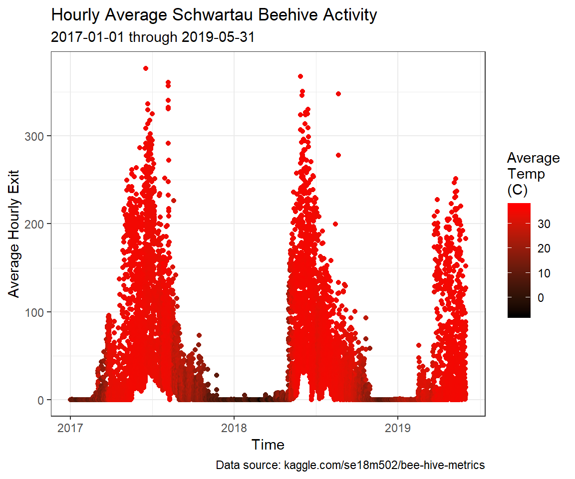
There is a pretty thick line of inactivity at all temperatures, though, which makes me wonder if the beehive has been active the whole time it was being observed. Let’s make a plot of activity over time.
joined_table %>%
  ggplot(aes(x = timestamp, y = mean_exit_flow, color = mean_temp)) +
  geom_point() +
  labs(title = "Hourly Average Schwartau Beehive Activity",
       subtitle = "2017-01-01 through 2019-05-31",
       caption = "Data source: kaggle.com/se18m502/bee-hive-metrics",
       color = "Average\nTemp\n(C)") +
  xlab("Time") +
  ylab("Average Hourly Exit") +
  scale_colour_gradient(low = "black", high = "red") +
  theme_bw()
As I expected, the beehive activity is function of both temperature and time of year. Also, there are some times of year where there are bees exiting the hive twenty-four hours per day.
There you have it! While there’s nothing wrong with using Excel, especially when it’s the medium that your colleagues are familiar with, R is much faster, and more reproducible and flexible. I can easily read through the code that I just wrote and follow what’s happening, but when I get an Excel workbook with similar calculations, it takes quite a bit of time to figure out what’s going on.